Using Microsoft Excel to Calculate FTE and Leave Entitlement

Full Time Equivalence (FTE) is an important tool within human resource management. FTE allows an organisation to normalise employee contractual hours against a base set of full-time hours. In resource planning this can be used (in part) to understand how a full-time role can be represented as multiple part time roles. FTE can also be used to demonstrate parity between full and part time members of staff by allowing benefits, such as paid leave to be calculated accurately.

This spreadsheet provides a simple and basic means of calculating FTE using multiple sets of full time and contractual hours. Leave entitlements can also be calculated by setting the appropriate values. In HR software systems, such as People Inc., FTE calculations play an important role. These types of system are able to pro rate leave entitlement accurately for new starters and leavers as well as accommodating multiple changes of FTE within an absence year.

Defining the Full Time Hours

An organisation will define through some means an amount of time which constitutes their full-time hours. They may need to do this multiple times depending on the type of work being undertaken; for example, a full-time office worker may be considered full time if they work 37.5 hours whilst a factory worker may need to work 45 hours. These full-time hours are then split over a number of days in a week or over a period of weeks.

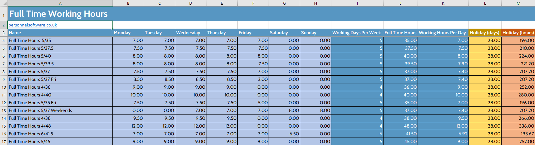
In Excel create a new sheet, in this example the sheet has been named ‘Full Time Working Hours’ and contains 17 rows in total. To be consisted with the formula used in this example the first two rows are used for the title of the sheet and a url. The third row is used as the header row for the following columns:

• A Name – A friendly name for the set of full-time hours
• B Monday – The standard working hours on a Monday
• C Tuesday – The standard working hours on a Tuesday
• D Wednesday – The standard working hours on a Wednesday
• E Thursday – The standard working hours on a Thursday
• F Friday – The standard working hours on a Friday
• G Saturday – The standard working hours on a Saturday
• H Sunday – The standard working hours on a Sunday
• I Working Days Per Week – How many days in the week work is performed
• J Full Time Hours – The total number of hours worked in a week
• K Working Hours Per Day – The average number of hours worked on each work day
• L Holiday (days) – The holiday / leave entitlement based in days
• M Holiday (hours) – The holiday / leave entitlement based in days

Columns A to H do not contain any formula. Column A will contain text only, columns B – H and J – M should be formatted to contain decimal numbers to 2 decimal places. Column I will contain whole numbers only.

• Column I calculation – Working Days per Week

  Starting from row 4 and copying down the formula in this column will look at the values in columns B, C, D, E, F, G and H. If the value in any of those columns in greater than zero then it will be counted as a working day.

  The formula for this is:

  =IF(B4 > 0, 1, 0) + IF(C4 > 0, 1, 0) + IF(D4 > 0, 1, 0) + IF(E4 > 0, 1, 0) + IF(F4 > 0, 1, 0) + IF(G4 > 0, 1, 0) + IF(H4 > 0, 1, 0)

• Column J calculation – Full Time Hours

  Again, starting from row 4 and copying down, this formula will sum the columns B, C, D, E, F, G and H. This will be the total number of hours worked in a week.

  The formula for this is:

  =SUM(B4:H4)

• Column K calculation – Working Hours Per Day

  This column will calculate the average number of workings which occur on each working day. This is done by dividing the working hours (column J) by the number of days worked (column I).

  The formula for this is:

  =IF(AND(I4>0,J4>0),J4/I4,0)

  Note that this formula is checking if column and I and J have a value using the AND function before attempting the division.

• Column M calculation – Holiday (hours) (Optional)

  This column calculates the equivalent number of hours for the number of days entered in column L.

  The formula for this is:

  =L4*K4

Column L contains the holiday in days, Column K contains the average number of working hours per day worked in the week.

Defining the Contractual Hours

Contractual hours are recorded in a similar way to full time hours but relate to individual employees.

Create a new sheet in the Excel work book which contain the Full Time Working Hours sheet described above. In this example we have named the sheet ‘Employee Contractual Hours’. To be consistent with this example, the first three rows are used for the title of the sheet, a url and the column headings. As this sheet may contain a large number of rows the heading can be fixed by selecting them and using Freeze Panes in the View tab of Excel.

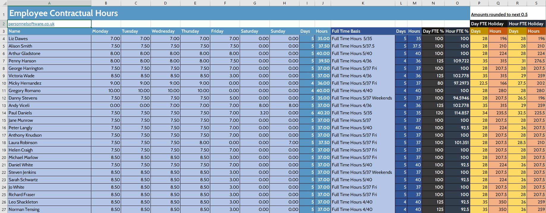
Define the following column headings in row 3 of the sheet:

• A Name – This is the name of the employee
• B Monday – The contractual hours for a Monday
• C Tuesday – The contractual hours for a Tuesday
• D Wednesday – The contractual hours for a Wednesday
• E Thursday – The contractual hours for a Thursday
• F Friday – The contractual hours for a Friday
• G Saturday – The contractual hours for a Saturday
• H Sunday – The contractual hours for a Sunday
• I Days – How many days in the week which are worked
• J Hours – How many hours are working in the week in total
• K Full Time Basis – This is a drop down which chooses which set of full-time hours the contract is based on.
• L Days – A lookup field showing the full-time working days for this set of full-time hours
• M Hours – A lookup field showing the full-time working hours for this set of full-time hours
• N Day FTE % – The employees FTE based on days worked in the week
• Hour FTE % – The employees FTE based on the hours working in the week
• P Days – The number of days leave based on the employee’s day-based FTE
• Q Hours – The number of hours leave based on the employee’s day-based FTE
• R Days – The number of days leave based on the employee’s hour-based FTE
• S Hours – The number of hours leave based on the employee’s hour-based FTE

Again, in this sheet columns A to H do not contain any formula. Column A should be formatted for text. Columns B to H, and J will hold decimal numbers to two decimal places. Column I will hold whole numbers.

• Column I calculation – Days

  This column works exactly the same way as Column I in the ‘Full Time Working Hours’ sheet. Again, starting from row 4 and copying down the formula in this column will look at the values in columns B, C, D, E, F, G and H. If the value in any of those columns in greater than zero then it will be counted as a day.

  The formula for this is:

  =IF(B4 > 0, 1, 0) + IF(C4 > 0, 1, 0) + IF(D4 > 0, 1, 0) + IF(E4 > 0, 1, 0) + IF(F4 > 0, 1, 0) + IF(G4 > 0, 1, 0) + IF(H4 > 0, 1, 0)

• Column J calculation – Hours

  A above, this column works the same way as Column J in the ‘Full Time Working Hours’ sheet, starting from row 4 and copying down, this formula will sum the columns B, C, D, E, F, G and H. This will be the total number of contractual hours in a week.

  The formula for this is:

  =SUM(B4:H4)

• Column K calculation – Full Time Basis

  This column will look up the values in column A of the ‘Full Time Working Hours’ sheet and generate a drop-down list. Choosing a value from the list will set the full-time hours which the contractual hours will be compared to.

  For more help on creating a drop down list in Excel please see this help article by Microsoft.

  Alternatively, you can manually enter the name of the full-time hours (exactly as it appears in the other sheet).

• Column L calculation – Days

  Based on the value selected in column K the full-time working days will be shown here.

  The formula for this is:

  =IF(AND(VLOOKUP(K4,'Full Time Working Hours'!$A$4:$M$17,9,FALSE)>0, (I4>0)),VLOOKUP(K4,'Full Time Working Hours'!$A$4:$M$17,9,FALSE),0)

• Column M calculation – Hours

  This column works the same way as column L above but looks up the full-time working hours.

  The formula for this is:

  =IF(AND(VLOOKUP(K4,'Full Time Working Hours'!$A$4:$J$17,10,FALSE)>0, (J4>0)),VLOOKUP(K4,'Full Time Working Hours'!$A$4:$J$17,10,FALSE),0)

• Column N calculation – Day FTE %

  The day FTE is a comparison of the full-time working days and the employee working days. In this example this is calculated as a percent, dividing by 100 will calculate the equivalence. Note that this formula does not attempt to round the result.

  The formula for this is:

  =IF(AND(I4>0, L4>0), (100 * I4) / L4, 0)

• Column O calculation – Hour FTE %

  The hour FTE is a comparison of the full-time hours and the total contractual hours. Again, in this example the FTE is calculated as a percentage, divide this by 100 to get the equivalence. This formula does not attempt to round the result.

  The formula for this is:

  =IF(AND(J4>0, M4>0), (100 * J4) / M4, 0)

• Column P calculation – Holiday Days (based on day-based FTE)

  In this column the leave entitlement value in the ‘Full Time Working Hours’ sheet is looked up and then factored by the FTE defined in column N. The result is rounded up to the nearest 0.5.

  The formula for this is:

  =CEILING(IF($N4>0, ($N4 / 100) * IF(AND(VLOOKUP($K4,'Full Time Working Hours'!$A$4:$M$17,12,FALSE)>0, ($I4>0)),VLOOKUP($K4,'Full Time Working Hours'!$A$4:$M$17,12,FALSE),0), 0), 0.5)

• Column Q calculation – Holiday Hours (based on day-based FTE)

  This column works in the same way as column P, looking up the leave entitlement in the ‘Full Time Working Hours’ sheet. This column will reference the entitlement defined as hours. The result is rounded up to the nearest 0.5.

  The formula for this is:

  =CEILING(IF($N4>0, ($N4 / 100) * IF(AND(VLOOKUP($K4,'Full Time Working Hours'!$A$4:$M$17,13,FALSE)>0, ($I4>0)),VLOOKUP($K4,'Full Time Working Hours'!$A$4:$M$17,13,FALSE),0), 0), 0.5)

• Column R calculation – Holiday Days (based on hour-based FTE)

  Again, this column is similar to column P however rather than using the Day FTE value from column N it uses the Hour FTE from column O. The result is rounded up to the nearest 0.5.

  The formula for this is:

  =CEILING(IF($O4>0, ($O4 / 100) * IF(AND(VLOOKUP($K4,’Full Time Working Hours’!$A$4:$M$17,12,FALSE)>0, ($I4>0)),VLOOKUP($K4,’Full Time Working Hours’!$A$4:$M$17,12,FALSE),0), 0), 0.5)

• Column S calculation – Holiday Days (based on hour-based FTE)

  This column works in the same way as Column Q but uses the Hour FTE value found in column O. The result is rounded up to the nearest 0.5.

  The formula for this is:

  =CEILING(IF($O4>0, ($O4 / 100) * IF(AND(VLOOKUP($K4,'Full Time Working Hours'!$A$4:$M$17,13,FALSE)>0, ($I4>0)),VLOOKUP($K4,'Full Time Working Hours'!$A$4:$M$17,13,FALSE),0), 0), 0.5)

Why Calculate FTE Twice (in days and hours)?

The different approaches are used in different situations. Day based FTE can be much simpler for calculating time off, one date will equate to one day off. The disadvantage is that this is highly inaccurate, an employee working five hours on one day of the week and nine on another has significant variation based on which day they take off. Working in hour-based FTE provides a greater level of accuracy, days off equate to working days lost rather than dates. A date may then represent less than or more than one working day depending on that day’s contractual hours

Formulas & Functions

• Calculating the FTE

  The formula for FTE is

  Contractual hours / full time hours = Full Time Equivalence (hours)

  Working days / full time days = Full Time Equivalence (days)

  To convert the equivalence to a percentage multiply by 100.

• Calculating Entitlements

  To proportionally award leave entitlements based on FTE you can use the following formula:

  Full Time Leave Entitlement * Full Time Equivalence = Leave Entitlement

  Full Time Leave Entitlement * (Full Time Equivalence Percent / 100) = Leave Entitlement

• The Excel IF function

  In Excel the IF function can be used to insert one of two values based on a user defined condition:

  =IF(userdefinedcondition, trueoutcome, falseoutcome)

  userdefinedcondition must evaluate to a Boolean (true / false) value.

  trueoutcome is the value which will appear if the userdefinedcondition evaluates to true. The value can be entered literally or it can be derived from an additional formula.

  falseoutcome worked in the same way as trueoutcome and will be used if userdefinedconditionevaluates to false.

• The Excel Sum function

  =SUM(startcell, endcell)

  startcell is first cell in the range, endcell is the last. An alternative option is to use Excels auto sum feature and select the range of cells to total.

• The Excel And function

  The And function allows Boolean values (taken from cells or a formula) to be evaluated.

  =AND(firstboolean,secondboolean)

  AND will return true if both firstboolean and secondboolean evaluate to true. If either (or both) were to evaluate to false then the and function will return false.

• Safe Division

  It is not possible to divide by zero. In order to be certain of the outcome of a calculation it must be written in such a way that this risk is accounted for.

• The Excel VLookup function

  VLookups match the value in one cell with the value in another cell in a specified range of cells. From this range it is possible to select a value from a column in that range.

  =VLOOKUP(referencecell, lookupcellrange, columnnumber, exactmatch)

  The referencecell is the cell which contain the key value that will be searched for. The loookupcellrange is where the value should be search for, the first column of the range is where the referencecell value is searched for. The lookupcellrange will define a one or more columns, rather than referring to them by their cell co-ordinates the columns will be numbered from 1 onwards. The columnnumber defines which column the value for this cell will be found in. The exactmatch parameter specifies if the key value in the referencecell toggles if the value must match exactly (false) or if partial matches are acceptable (true).

• The Excel Ceiling function

  Ceiling is a function used to round a value to the next increment (as apposed to the Floor function which will round down).

  =CEILING(unroundedvalue, increment)

  The unreoundedvalue could be a formula, cell value or a literal value. The increment defines the rounding to apply, 0.5 for half, 0.75 for three quarters etc.

More Information

If you would like more information about how People Inc. generates and manages holiday allowances, and how it can help manage staff using their FTE, please contact us on 01908 265111, or click the button below to request a call-back.

Related Features

The People Inc. system provides extensive functionality to help manage employee absence. Links to some examples are provided below:

Absence Update

Additional People Inc. features designed to help manage holidays and other forms of absence.

Absence Year End

Advice and guidance on the year-end activities related to People Inc. absence management.

Absence Features

A summary of the absence features offered by the People Inc. system, and the ESS module.

Discover more about these topics

• FTE
• Pro Rata
• Full Time Hours
• Excel
• Contractual Hours
• Leave

External Resources

Listed below are some links to additional absence-related information. The links go to pages on external websites. These links are given for reference only.

• Checking Holiday Entitlement (www.acas.org.uk) - External Link.

• UK Bank Holidays (www.gov.uk) - External Link.

• Covid-19 rules on carry over (www.gov.uk) - External Link.